Permutation Importance Documentation

scikit-explain includes single-pass, multi-pass, second-order, and grouped permutation importance , respectively. In this notebook, we highlight how to compute these methods and plot their results. In the first set of examples, two tree-based models (random forest and gradient-boosting) and logistic regression from scikit-learn were trained on a portion of the road surface temperature data from Handler et al. (2020). The goal is to predict whether road surface temperatures will be above or below freezing (32 F) in the next hour. This dataset has 100 K examples with a class skew of 39%.

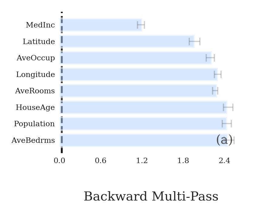
A regression-based example is also shown using the Californina housing dataset available in scikit-learn.

import sys, os
sys.path.insert(0, os.path.dirname(os.getcwd()))

plotting_config is a python script that contains plotting variables for the built-in skexplain dataset. If you execute this notebook in another directory, you’ll have to copy over that script.

import skexplain
import plotting_config

# Loading the training data and pre-fit models for the classification problem
estimators = skexplain.load_models()
X,y = skexplain.load_data()

print(estimators)
print(f'X Shape : {X.shape}')
print(f'y Skew : {y.mean()*100}%')

[('Random Forest', RandomForestClassifier(min_samples_leaf=5, n_estimators=200, n_jobs=5)), ('Gradient Boosting', GradientBoostingClassifier()), ('Logistic Regression', LogisticRegression(C=1))]
X Shape : (100000, 30)
y Skew : 39.173%

Computing Permutation Importance

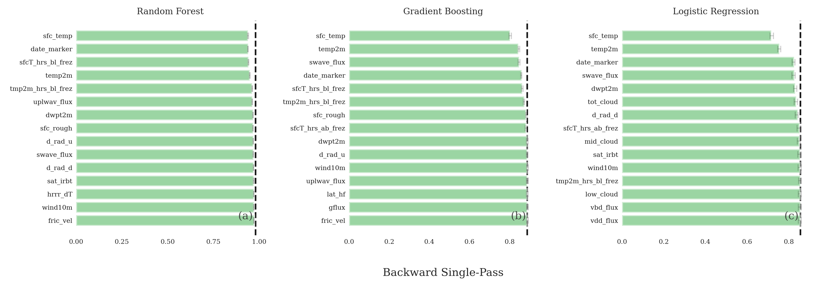
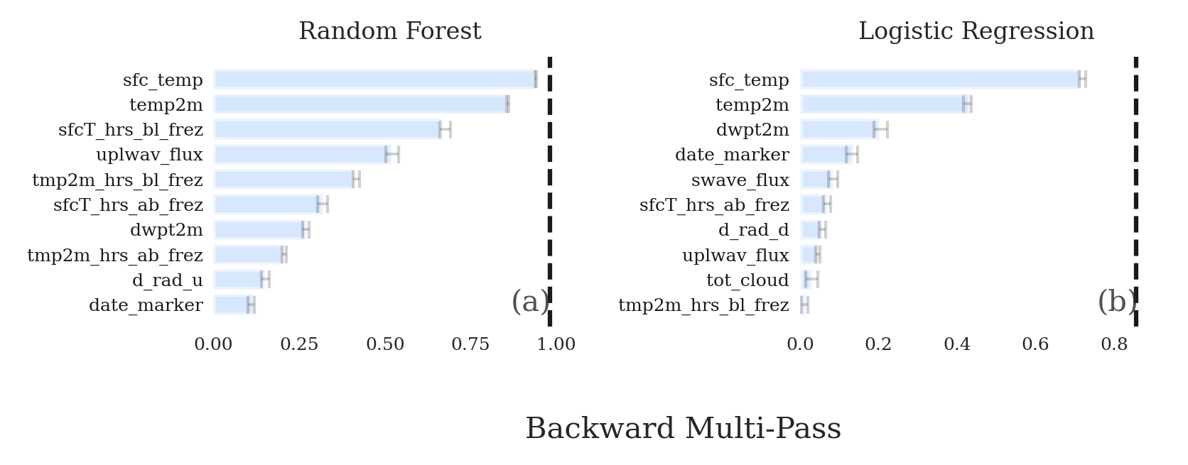
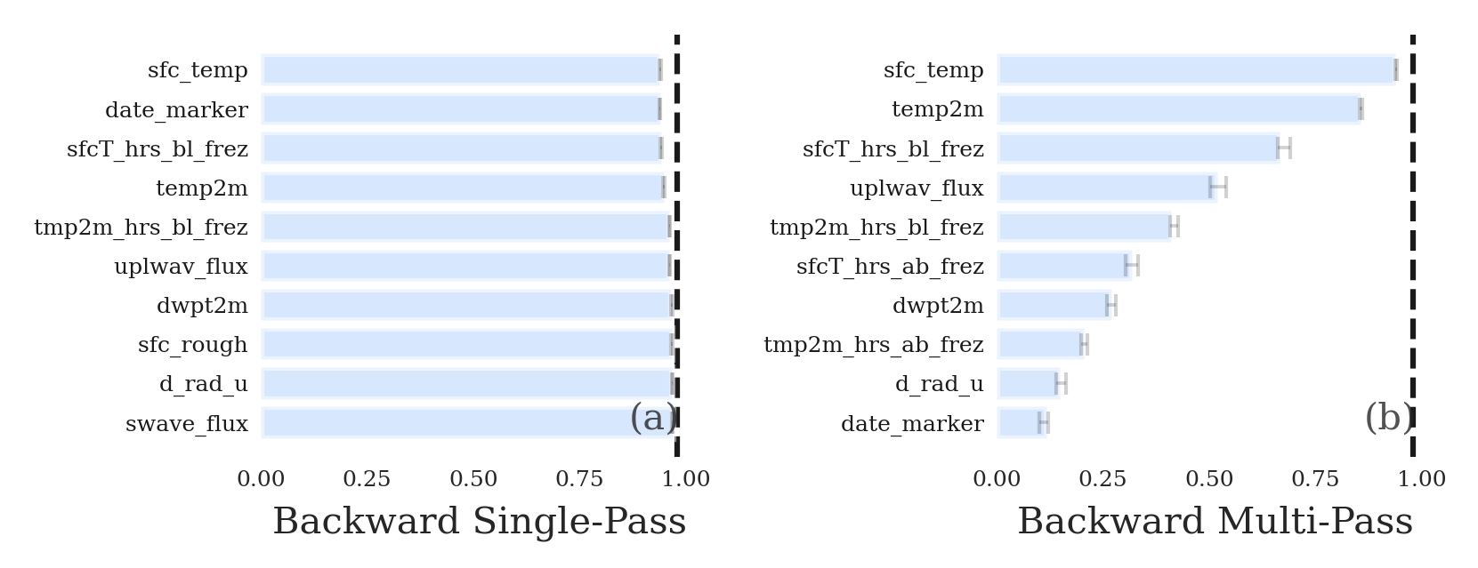
Feature/predictor ranking is often a first step in model explainability and a popular model-agnostic approach is the permutation importance method. In this method the data for each feature is permuted (shuffled) and the permuted feature associated the greatest decrease in model performance (based on some error metric) is deemed the most important (and each feature is ranked subsequently). This describes what is known as the backward single-pass permuation importance method (McGovern et al. 2019; Fig 1 for an illustration). This method is appropriate for datasets with independent features (where little to no correlations exist between features). For datasets with physical or statistically dependent features, we can extend the single-pass method to permuted multiple features (known as the multi-pass permutation method; Lakshmanan et al. 2015, JOAT; see Fig.2) where the top feature remains permuted before assessing the second most important predictor, and so on for the third predictor and beyond. By keeping features permuted, it ought to break the interfeature correlations.

skexplain.calc_permutation_importance requires the following args:

• n_vars, the number of predictor to compute for the multi-pass method.

• evaluation_fn, the error function used to assess loss of skill.

  • mintpy has 5 built-in error metrics for evaluating predictor importance:

    • Area under the Curve ('auc')

    • Area under the Precision-Recall Curve ('aupdrc')

    • Normalized Area under the Performance Diagram Curve ('norm_aupdc')

    • Brier Skill Score ('bss')

    • Mean Square Error ('mse')

• n_permute, number of times to repeat permutations for confidence intervals

• subsample, can be a float between 0-1 or an integer, which is interpreted as the percentage of examples or exact number of random samples to use, respectively.

• n_jobs, number of processor to run the script on.

  • Could be the exact number or percentage of the total available to use (0-1) similar to subsample

• verbose, allows for a print out of the progress.

• random_state, Pass an int to get reproducible results across function calls.

• direction, Whether features are progressively unpermuted ('forward') or features are left permuted for second-, third-most important features ('backward'). The results are often not identical.

Note: evaluation_fn can also be any user-defined function of the form evaluation_fn(targets,predictions) where a single value is returned. However, when using your own function, then you must also set the scoring strategy argument. If a metric is positively-oriented (a higher value is better), then set scoring_strategy = "minimize" and if it is negatively-oriented-oriented (a lower value is better), then set scoring_strategy = "maximize".

In this example, we want to know the top 10 predictors for each ML model. We are using normalized area under the precision-recall curve (NAUPDC; Flora et al. 2021, Miller et al. 2022) as the error metric. To produce confidence intervals, we are using 5 bootstrap iterations (kept small for demostration purposes, but should typically be >30). The multipass permutation importance method can be computationally expensive for larger datasets. Thus, we’ve included a method to skexplain to store the results for later use. The results are stored in xarray.Datasets and saved as netcdf files.

explainer = skexplain.ExplainToolkit(estimators,X=X, y=y,)

explainer.set_plotting_config(
    display_feature_names=plotting_config.display_feature_names,
    display_units=plotting_config.display_units,
    feature_colors=plotting_config.color_dict,
)

%time
results = explainer.permutation_importance(
                                           n_vars=10,
                                           evaluation_fn='norm_aupdc',
                                           n_permute=5,
                                           subsample=0.1,
                                           n_jobs=8,
                                           verbose=True,
                                           random_seed=42,
                                           direction='backward',
                                              )

# Save the permutation importance results as a netcdf file using the bulit-in function within scikit-explain
explainer.save(fname='../tutorial_data/multipass_importance_naupdc.nc', data=results)

CPU times: user 5 µs, sys: 4 µs, total: 9 µs
Wall time: 19.3 µs

Perm. Imp.: 100%|█████████████████████████████████████████████████████████████████████████████████████████████████████████| 10/10 [00:47<00:00,  4.72s/it]
Perm. Imp.: 100%|█████████████████████████████████████████████████████████████████████████████████████████████████████████| 10/10 [00:39<00:00,  3.91s/it]
Perm. Imp.: 100%|█████████████████████████████████████████████████████████████████████████████████████████████████████████| 10/10 [00:50<00:00,  5.07s/it]

Loading saved permutation importance results

There are I/O methods built into scikit-explain that allows for loading and saving ExplainToolikit results. For example, we might want one script for computing the explainability results and another for loading them to plot the results. To do so, we initialize an empty ExplainToolkit and call the load method. There are attributes saved in each output netCDF file that are used as an attributes for ExplainToolkit, which makes using scikit-explain more streamlined. Though it is not demonstrated here, you can also pass a list of filenames and the datasets are merged into one when being loaded.

# Instantiate an empty explainer class.
explainer = skexplain.ExplainToolkit()
# Load the results file; gets load as a class attribute
results = explainer.load(fnames='../tutorial_data/multipass_importance_naupdc.nc')

Plotting Single-Pass Permutation Importance for a Single Model

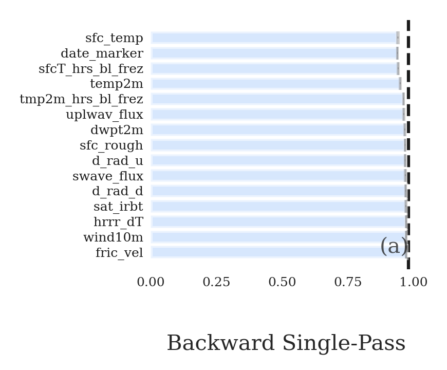
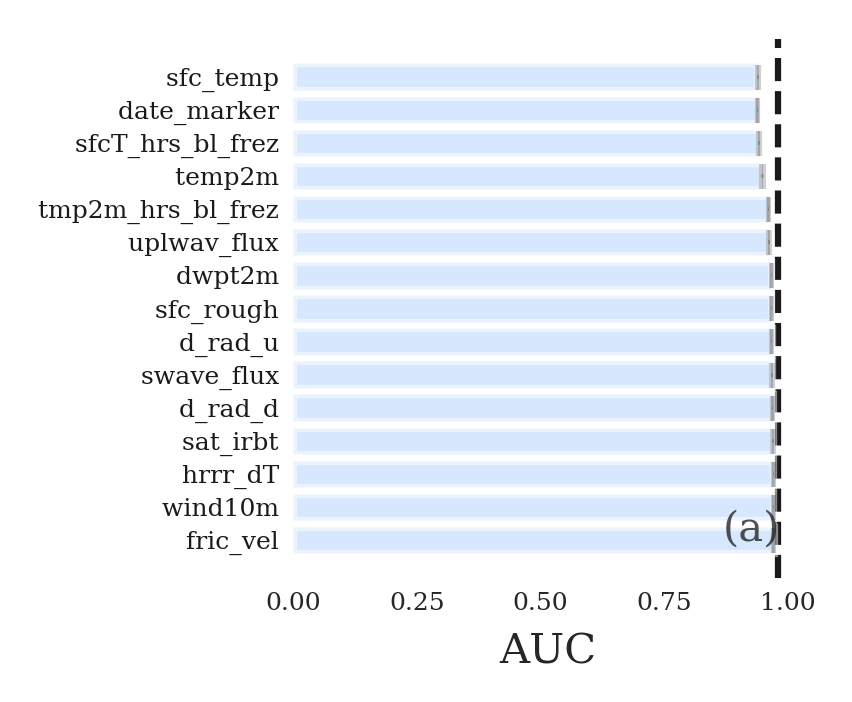
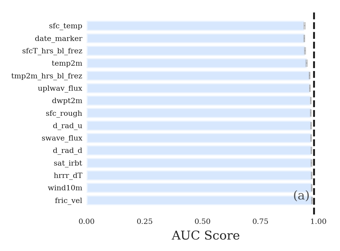
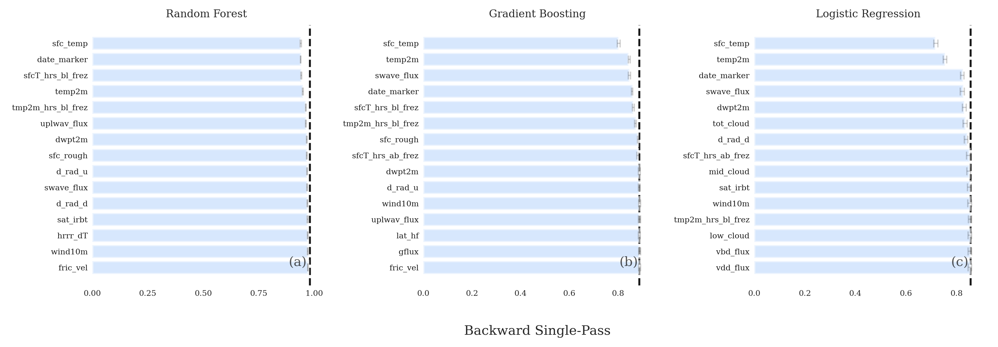
The first iteration of the multi-pass permutation method is the single-pass method and is therefore saved by default. Feature ranking plotting in scikit-explain is highly flexible, so if we want show multiple panels, then we need to declare what to show in each panel (i.e., (method, estimator name)). For example, to only plot the singlepass results from the random forest, we set panels=[('singlepass', 'Random Forest')]. The single-pass method ranks all features, so for readability, you can set num_vars_to_plot (default=15).

Note : Importance scores for the backward method are determined based on deviation from the original score. The original score is shown as the vertical dashed line.

fig = explainer.plot_importance(data=results,
                                panels=[('backward_singlepass', 'Random Forest')],
                                num_vars_to_plot=15,
                                 )

Changing the X-axis label

By default, skexplain uses the method name for the X-axis label. We can use the arg x_labels for custoum X-axis labelling. In this case, we set it to “AUC”. When we increase the number of panels, x_labels should be a list of labels for each panel.

fig = explainer.plot_importance(data=results,
                                panels=[('backward_singlepass', 'Random Forest')],
                                num_vars_to_plot=15,
                                xlabels = ['AUC']
                                 )

Using a custom axes object

By default, scikit-explain will internally create matplotlib.Axes object and label them for scientific publication quality. To avoid this, the user can send in their own axes object

import matplotlib.pyplot as plt
fig, ax = plt.subplots(dpi=300, figsize=(4,3))

fig = explainer.plot_importance(data=results,
                                panels=[('backward_singlepass', 'Random Forest')],
                                num_vars_to_plot=15,
                                xlabels = ['AUC'],
                                ax=ax
                                 )
ax.set_xlabel('AUC Score')

Text(0.5, 44.749999999999986, 'AUC Score')

Plotting Single-Pass Permutation Importance for Multiple Models

We computed permutation importance results for 3 different ML models and we can display them in a single plot by adding to the panels arg. In some cases, the default figure size might produce less than desirable results. We can pass in the figsize arg to alter the figure size.