ExplainToolkit

• ExplainToolkit

class skexplain.main.explain_toolkit.ExplainToolkit(estimators=None, X=Empty DataFrame Columns: [0] Index: [], y=array([], dtype=float64), estimator_output=None, feature_names=None, seaborn_kws=None)

ExplainToolkit is the primary interface of scikit-explain. The modules contained within compute several explainability machine learning methods such as

Feature importance:

• permutation_importance

• ale_variance

Feature Attributions:

• ale

• pd

• ice

• shap

• local_contributions

Feature Interactions:

• interaction_strength

• ale_variance

• perm_based_interaction

• friedman_h_stat

• main_effect_complexity

• ale

• pd

Additionally, there are corresponding plotting modules for each method, which are designed to produce publication-quality graphics.

Note

ExplainToolkit is designed to work with estimators that implement predict or predict_proba.

Caution

ExplainToolkit is only designed to work with binary classification and regression problems. In future versions of skexplain, we hope to be compatiable with multi-class classification.

Parameters

• estimators (list of tuples of (estimator name, fitted estimator)) – Tuple of (estimator name, fitted estimator object) or list thereof where the fitted estimator must implement predict or predict_proba. Multioutput-multiclass classifiers are not supported.

• X ({array-like or dataframe} of shape (n_samples, n_features)) – Training or validation data used to compute the IML methods. If ndnumpy.array, must specify feature_names.

• y ({list or numpy.array} of shape (n_samples,)) – The target values (class labels in classification, real numbers in regression).

• estimator_output ("raw" or "probability") – What output of the estimator should be explained. Determined internally by ExplainToolkit. However, if using a classification model, the user can set to “raw” for non-probabilistic output.

• feature_names (array-like of shape (n_features,), dtype=str, default=None) – Name of each feature; feature_names[i] holds the name of the feature with index i. By default, the name of the feature corresponds to their numerical index for NumPy array and their column name for pandas dataframe. Feature names are only required if X is an ndnumpy.array, a it will be converted to a pandas.DataFrame internally.

• seaborn_kws (dict, None, or False (default is None)) –

  Arguments for the seaborn.set_theme(). By default, we use the following settings.

  custom_params = {“axes.spines.right”: False, “axes.spines.top”: False} sns.set_theme(style=”ticks”, rc=custom_params)

  If False, then seaborn settings are not used.

Raises

• AssertError – Number of estimator objects is not equal to the number of estimator names given!

• TypeError – y variable must be numpy array or pandas.DataFrame.

• Exception – Feature names must be specified if X is an numpy.array.

• ValueError – estimator_output is not an accepted option.

ale(features=None, n_bins=30, n_jobs=1, subsample=1.0, n_bootstrap=1, random_seed=42, class_index=1)

Compute the 1D or 2D centered accumulated local effects (ALE) 9 10. For categorical features, simply set the type of those features in the dataframe as category and the categorical ALE will be computed.

References

9

https://christophm.github.io/interpretable-ml-book/ale.html

10

Apley, D. W., and J. Zhu, 2016: Visualizing the Effects of Predictor Variables in Black Box Supervised Learning Models. ArXiv.

Parameters

• features (string or list of strings or 'all') – Features to compute the PD for. if ‘all’, the method will compute the ALE for all features.

• n_bins (integer (default=30)) – Number of bins used to compute the ALE for. Bins are decided based on percentile intervals to ensure the same number of samples are in each bin.

• n_jobs (float or integer (default=1)) –

  • if integer, interpreted as the number of processors to use for multiprocessing

  • if float, interpreted as the fraction of proceesors to use for multiprocessing

• subsample (float or integer (default=1.0)) –

  • if value between 0-1 interpreted as fraction of total X to use

  • if value > 1, interpreted as the absolute number of random samples of X.

• n_bootstrap (integer (default=1; no bootstrapping)) – Number of bootstrap resamples for computing confidence intervals on the ALE curves.

Returns

results – ALE result dataset

Return type

xarray.DataSet

Raises

Exception – Highly skewed data may not be divisable into n_bins given. In that case, calc_ale uses the max bins the data can be divided into. But a warning message is raised.

Examples

>>> import skexplain
>>> estimators = skexplain.load_models() # pre-fit estimators within skexplain
>>> X, y = skexplain.load_data() # training data
>>> # Set the type for categorical features and ExplainToolkit with compute the
>>> # categorical ALE.
>>> X = X.astype({'urban': 'category', 'rural':'category'})
>>> explainer = skexplain.ExplainToolkit(estimators=estimators
...                             X=X,
...                             y=y,
...                            )
>>> ale = explainer.ale(features='all')

ale_variance(ale, features=None, estimator_names=None, interaction=False, method='ale')

Compute the standard deviation (std) of the ALE values for each features in a dataset and then rank by the magnitude. A higher std(ALE) indicates a greater expected contribution to an estimator’s prediction and is thus considered more important. If interaction=True, then the method computes a similar method for the 2D ALE to measure the feature interaction strength.

This method is inspired by the feature importance and interaction methods developed in Greenwell et al. (2018) 4.

Parameters

• ale (xarray.Dataset) – Results of ale() for features.

• features ('all', string, list of strings, list of 2-tuples) – Features to compute the ALE variance for. If set to 'all', it is computed for all features. If interaction=True, then features must be a list of 2-tuples for computing the interaction between the set of feature combinations.

• estimator_names (string, list of strings) – If using multiple estimators, you can pass a single (or subset of) estimator name(s) to compute the ALE variance for.

• interaction (boolean) –

  • If True, it computes the feature interaction strength

  • If False, compute the feature importance

Returns

results_ds – ALE variance results. Includes both the rankings and scores.

Return type

xarray.Dataset

References

4

Greenwell, B. M., B. C. Boehmke, and A. J. McCarthy, 2018: A Simple and Effective estimator-Based Variable Importance Measure. Arxiv,.

Examples

>>> import skexplain
>>> import itertools
>>> # pre-fit estimators within skexplain
>>> estimators = skexplain.load_models()
>>> X, y = skexplain.load_data() # training data
>>> explainer = skexplain.ExplainToolkit(estimators=estimators,
...                             X=X,
...                             y=y,
...                            )
>>> ale = explainer.ale(features='all', n_bins=10, subsample=1000, n_bootstrap=1)
>>> # Compute 1D ALE variance
>>> ale_var_results = explainer.ale_variance(ale)
>>> print(ale_var_results)
<xarray.Dataset>
Dimensions:    (n_bootstrap: 1, n_vars_ale_variance: 30)
Dimensions without coordinates: n_bootstrap, n_vars_ale_variance
Data variables:
    ale_variance_rankings__Random Forest        (n_vars_ale_variance) <U17 'r...
    ale_variance_scores__Random Forest          (n_vars_ale_variance, n_bootstrap) float64 ...
    ale_variance_rankings__Gradient Boosting    (n_vars_ale_variance) <U17 'u...
    ale_variance_scores__Gradient Boosting      (n_vars_ale_variance, n_bootstrap) float64 ...
    ale_variance_rankings__Logistic Regression  (n_vars_ale_variance) <U17 'r...
    ale_variance_scores__Logistic Regression    (n_vars_ale_variance, n_bootstrap) float64 ...
Attribute:
    estimator_output:  probability
    estimators used:   ['Random Forest', 'Gradient Boosting', 'Logistic Regre...
    n_multipass_vars:  5
    method:            ale_variance
    direction:         backward
    evaluation_fn:     sigma_ale
    dimension:         1D
    features used:     ['dllwave_flux', 'dwpt2m', 'fric_vel', 'gflux', 'high_...
    estimator output:  probability
    interaction:       False

>>> #Typical, we only want to evaluate the feature interactions for
>>> # the most important features
>>> important_vars = ['sfc_temp', 'temp2m', 'sfcT_hrs_bl_frez', 'tmp2m_hrs_bl_frez',
...   'uplwav_flux']
>>> # Create all possible combinations
>>> important_vars_2d = list(itertools.combinations(important_vars, r=2))
>>> #For the 2D ALE variance to measure feature interaction strength
>>> ale_2d = explainer.ale(features=important_vars_2d, n_bins=10,
...              subsample=1000, n_bootstrap=1)
>>> # Compute 2D ALE variance
>>> ale_var_results = explainer.ale_variance(ale_2d, features=important_vars_2d,
...                    interaction=True)
>>> print(ale_var_results)
<xarray.Dataset>
Dimensions:   (n_bootstrap: 1, n_vars_ale_variance_interactions: 10)
Dimensions without coordinates: n_bootstrap, n_vars_ale_variance_interactions
Data variables:
    ale_variance_interactions_rankings__Random Forest        (n_vars_ale_variance_interactions) <U35 ...
    ale_variance_interactions_scores__Random Forest          (n_vars_ale_variance_interactions, n_bootstrap) float64 ...
    ale_variance_interactions_rankings__Gradient Boosting    (n_vars_ale_variance_interactions) <U35 ...
    ale_variance_interactions_scores__Gradient Boosting      (n_vars_ale_variance_interactions, n_bootstrap) float64 ...
    ale_variance_interactions_rankings__Logistic Regression  (n_vars_ale_variance_interactions) <U35 ...
    ale_variance_interactions_scores__Logistic Regression    (n_vars_ale_variance_interactions, n_bootstrap) float64 ...
Attribute:
    estimator_output:  probability
    estimators used:   ['Random Forest', 'Gradient Boosting', 'Logistic Regre...
    n_multipass_vars:  5
    method:            ale_variance
    direction:         backward
    evaluation_fn:     Interaction Importance
    dimension:         2D
    features used:     [('sfc_temp', 'temp2m'), ('sfc_temp', 'sfcT_hrs_bl_fre...
    estimator output:  probability
    interaction:       True

average_attributions(method=None, data=None, performance_based=False, n_samples=100, shap_kws=None, lime_kws=None, n_jobs=1)

Computes the individual feature contributions to a predicted outcome for a series of examples either based on tree interpreter (only Tree-based methods) , Shapley Additive Explanations, or Local Interpretable Model-Agnostic Explanations (LIME).

The primary difference between average_attributions and local_attributions is the performance-based determiniation of examples to compute the local attributions from. average_attributions can start with the full dataset and determine the top n_samples to compute explanations for.

Parameters

• method ('shap' , 'tree_interpreter', or 'lime' (default is None)) – Can use SHAP, treeinterpreter, or LIME to compute the feature attributions. SHAP and LIME are estimator-agnostic while treeinterpreter can only be used on select decision-tree based estimators in scikit-learn (e.g., random forests).

• data (dataframe or a list of dataframes, shape (n_examples, n_features) (Default is None)) – Local attribution data for each estimator. Results from explainer.local_attributions. If None, then the local attributions are computed internally.

• performance_based (boolean (default=False)) – If True, will average feature contributions over the best and worst performing of the given X. The number of examples to average over is given by n_samples

• n_samples (interger (default=100)) – Number of samples to compute average over if performance_based = True

Returns

results_df – For each example, contributions from each feature plus the bias The dataframe is nested by the estimator names and additional keys if performance_based=True.

Return type

nested pandas.DataFrame

Examples

>>> import skexplain
>>> import shap
>>> # pre-fit estimators within skexplain
>>> estimators = skexplain.load_models()
>>> X, y = skexplain.load_data() # training data
>>> # Only give the X you want contributions for.
>>> # In this case, we are using a single example.
>>> single_example = X.iloc[[0]]
>>> explainer = skexplain.ExplainToolkit(estimators=estimators
...                             X=single_example,
...                            )
>>> # Create a background dataset; randomly sample 100 X
>>> background_dataset = shap.sample(X, 100)
>>> contrib_ds = explainer.average_contributions(method='shap',
...                   background_dataset=background_dataset)

>>> # For the performance-based contributions,
>>> # provide the full set of X and y values.
>>> explainer = skexplain.ExplainToolkit(estimators=estimators
...                             X=X,
...                            y=y,
...                            )
>>> contrib_ds = explainer.average_contributions(method='shap',
...                   background_dataset=background_dataset,
...                   performance_based=True, n_samples=100)

friedman_h_stat(pd_1d, pd_2d, features, estimator_names=None, **kwargs)

Compute the second-order Friedman’s H-statistic for computing feature interactions 11 12. Based on equation (44) from Friedman and Popescu (2008) 12. Only computes the interaction strength between two features. In future versions of skexplain we hope to include the first-order H-statistics that measure the interaction between a single feature and the remaining set of features.

References

11

https://christophm.github.io/interpretable-ml-book/interaction.html

12(1,2)

Friedman, J. H., and B. E. Popescu, 2008: Predictive learning via rule ensembles. Ann Appl Statistics, 2, 916–954, https://doi.org/10.1214/07-aoas148.

Parameters

• pd_1d (xarray.Dataset) – 1D partial dependence dataset. Results of pd() for features

• pd_2d (xarray.Dataset) – 2D partial dependence dataset. Results of pd(), but 2-tuple combinations of features.

• features (list of 2-tuples of strings) – The pairs of features to compute the feature interaction between.

• estimator_names (string, list of strings (default is None)) – If using multiple estimators, you can pass a single (or subset of) estimator name(s) to compute the H-statistic for.

Returns

results_ds – The second-order Friedman H-statistic for all estimators.

Return type

xarray.Dataset

Examples

>>> import skexplain
>>> # pre-fit estimators within skexplain
>>> estimators = skexplain.load_models()
>>> X, y = skexplain.load_data() # training data
>>> explainer = skexplain.ExplainToolkit(estimators=estimators
...                             X=X,
...                             y=y,
...                            )
>>> pd_1d = explainer.pd(features='all')
>>> pd_2d = explainer.pd(features='all_2d')
>>> hstat = explainer.friedman_h_stat(pd_1d, pd_2d,)

get_important_vars(perm_imp_data, multipass=True, n_vars=10, combine=False)

Retrieve the most important variables from permutation importance. Can combine rankings from different estimators and only keep those variables that occur in more than one estimator.

Parameters

• perm_imp_data (xarray.Dataset) – Permutation importance result dataset

• multipass (boolean (defaults to True)) – if True, return the multipass rankings else returns the singlepass rankings

• n_vars (integer (default=10)) – Number of variables to retrieve if multipass=True.

• combine (boolean (default=False)) – If combine=True, n_vars can be set such that you only include a certain amount of top features from each estimator. E.g., n_vars=5 and combine=True means to combine the top 5 features from each estimator into a single list.

Examples

if combine=True

resultslist

List of top features from a different estimators.

if combine=False

resultsdict

keys are the estimator names and items are the top features.

Examples

>>> import skexplain
>>> # pre-fit estimators within skexplain
>>> estimators = skexplain.load_models()
>>> X, y = skexplain.load_data() # training data
>>> explainer = skexplain.ExplainToolkit(estimators=estimators
...                             X=X,
...                             y=y,
...                            )
>>> perm_imp_data = explainer.permutation_importance(
...                       n_vars=10,
...                       evaluation_fn = 'norm_aupdc',
...                       direction = 'backward',
...                       subsample=0.5,
...                       n_bootstrap=20,
...                       )
>>> important_vars = explainer.get_important_vars(perm_imp_data,
...        multipass=True, n_vars=5, combine=False)
...
>>> # set combine=True
>>> important_vars = explainer.get_important_vars(perm_imp_data,
...        multipass=True, n_vars=5, combine=True)

grouped_permutation_importance(perm_method, evaluation_fn, scoring_strategy=None, n_permute=1, groups=None, sample_size=100, subsample=1.0, n_jobs=1, clustering_kwargs={'n_clusters': 10})

The group only permutation feature importance (GOPFI) from Au et al. 2021 [1]_ (see their equations 10 and 11). This function has a built-in method for clustering features using the sklearn.cluster.FeatureAgglomeration. It also has the ability to compute the results over multiple permutations to improve the feature importance estimate (and provide uncertainty).

Original score = Jointly permute all features Permuted score = Jointly permuting all features except the considered group

Loss metrics := Original_score - Permuted Score Skill Score metrics := Permuted score - Original Score

Parameters

• perm_method ("grouped" or "grouped_only") –

  If "grouped", the features within a group are jointly permuted and other features are left unpermuted.

  If "grouped_only", only the features within a group are left unpermuted and other features are jointly permuted.

• evaluation_fn (string or callable) –

  evaluation/scoring function for evaluating the loss of skill once a feature is permuted. evaluation_fn can be set to one of the following strings:

  • "auc", Area under the Curve

  • "auprc", Area under the Precision-Recall Curve

  • "bss", Brier Skill Score

  • "mse", Mean Square Error

  • "norm_aupdc", Normalized Area under the Performance Diagram (Precision-Recall) Curve

  Otherwise, evaluation_fn can be any function of form, evaluation_fn(targets, predictions) and must return a scalar value

  When using a custom function, you must also set the scoring strategy (see below).

• scoring_strategy (string (default=None)) –

  This argument is only required if you are using a non-default evaluation_fn (see above)

  If the evaluation_fn is positively-oriented (a higher value is better), then set scoring_strategy = "minimize" (i.e., a lower score after permutation indicates higher importance) and if it is negatively-oriented- (a lower value is better), then set scoring_strategy = "maximize"

• n_permute (integer (default=1 for only one permutation per feature)) – Number of permutations for computing confidence intervals on the feature rankings.

• groups (dict (default=None)) – Dictionary of group names and the feature names or feature column indices. If None, then the feature groupings are determined internally based on feature clusterings.

• sample_size (integer (default=100)) – Number of random samples to determine the correlation for the feature clusterings

• subsample (float or integer (default=1.0 for no subsampling)) – if value is between 0-1, it is interpreted as fraction of total X to use if value > 1, interpreted as the number of X to randomly sample from the original dataset.

• n_jobs (interger or float (default=1; no multiprocessing)) – if integer, interpreted as the number of processors to use for multiprocessing if float between 0-1, interpreted as the fraction of proceesors to use for multiprocessing

• clustering_kwargs (dict (default = {'n_clusters' : 10})) – See https://scikit-learn.org/stable/modules/generated/sklearn.cluster.FeatureAgglomeration.html for details

Returns

• results (xarray.DataSet) – Permutation importance results. Includes the both multi-pass and single-pass feature rankings and the scores with the various features permuted.

• groups (dict) – If groups is None, then it returns the groups that were automatically created in the feature clustering. Otherwise, only results is returned.

References

1

Au, Q., J. Herbinger, C. Stachl, B. Bischl, and G. Casalicchio, 2021:

Grouped Feature Importance and Combined Features Effect Plot. Arxiv,.

Examples

>>> import skexplain
>>> # pre-fit estimators within skexplain
>>> estimators = skexplain.load_models()
>>> X, y = skexplain.load_data() # training data
>>> # Only compute for the first model
>>> explainer = skexplain.ExplainToolkit(estimators=estimators[0],
...                             X=X,
...                             y=y,
...                            )
>>> # Group only, the features within a group are the only one's left unpermuted
>>> results, groups = explainer.grouped_permutation_importance(
...                                          perm_method = 'grouped_only',
...                                          evaluation_fn = 'norm_aupdc',)
>>> print(results)
<xarray.Dataset>
     Dimensions:                        (n_vars_group: 10, n_bootstrap: 1)
     Dimensions without coordinates: n_vars_group, n_bootstrap
     Data variables:
         group_rankings__Random Forest  (n_vars_group) <U7 'group 3' ... 'group 4'
         group_scores__Random Forest    (n_vars_group, n_bootstrap) float64 0.4822...
     Attributes:
         estimators used:   ['Random Forest']
         estimator output:  probability
         estimator_output:  probability
         groups:            {'group 0': array(['d_rad_d', 'd_rad_u'], dtype=object...
         method:            grouped_permutation_importance
         perm_method:       grouped_only
         evaluation_fn:     norm_aupdc
>>> print(groups)
{'group 0': array(['d_rad_d', 'd_rad_u'], dtype=object),
'group 1': array(['high_cloud', 'lat_hf', 'mid_cloud', 'sfcT_hrs_ab_frez', 'date_marker'], dtype=object),
'group 2': array(['dllwave_flux', 'uplwav_flux'], dtype=object),
'group 3': array(['dwpt2m', 'fric_vel', 'sat_irbt', 'sfc_rough', 'sfc_temp',
'temp2m', 'wind10m', 'urban', 'rural', 'hrrr_dT'], dtype=object),
'group 4': array(['low_cloud', 'tot_cloud', 'vbd_flux', 'vdd_flux'], dtype=object),
'group 5': array(['gflux', 'd_ground'], dtype=object),
'group 6': array(['sfcT_hrs_bl_frez', 'tmp2m_hrs_bl_frez'], dtype=object),
'group 7': array(['swave_flux'], dtype=object),
'group 8': array(['sens_hf'], dtype=object),
'group 9': array(['tmp2m_hrs_ab_frez'], dtype=object)
}

ice(features, n_bins=30, n_jobs=1, subsample=1.0, n_bootstrap=1, random_seed=1)

Compute the indiviudal conditional expectations (ICE) 7.

References

7

https://christophm.github.io/interpretable-ml-book/ice.html

Parameters

• features (string or list of strings or 'all') – Features to compute the ICE for. if ‘all’, the method will compute the ICE for all features.

• n_bins (integer (default=30)) – Number of bins used to compute the ICE for. Bins are decided based on percentile intervals to ensure the same number of samples are in each bin.

• n_jobs (float or integer (default=1)) –

  • if integer, interpreted as the number of processors to use for multiprocessing

  • if float, interpreted as the fraction of proceesors to use for multiprocessing

• subsample (float or integer (default=1.0)) –

  • if value between 0-1 interpreted as fraction of total X to use

  • if value > 1, interpreted as the absolute number of random samples of X.

• n_bootstrap (integer (default=1; no bootstrapping)) – Number of bootstrap resamples for computing confidence intervals on the ICE curves.

Returns

results – Main keys are the user-provided estimator names while the sub-key are the features computed for. The items are data for the ICE curves. Also, contains X data (feature values where the ICE curves were computed) for plotting.

Return type

xarray.DataSet

Examples

>>> import skexplain
>>> # pre-fit estimators within skexplain
>>> estimators = skexplain.load_models()
>>> X, y = skexplain.load_data() # training data
>>> explainer = skexplain.ExplainToolkit(estimators=estimators,
...                             X=X,
...                             y=y,
...                            )
>>> ice_ds = explainer.ice(features='all', subsample=200)

interaction_strength(ale, estimator_names=None, **kwargs)

Compute the InterAction Strength (IAS) statistic from Molnar et al. (2019) 5. The IAS varies between 0-1 where values closer to 0 indicate no feature interaction strength.

Parameters

• ale (xarray.Dataset) – Results of ale(), but must be computed for all features

• estimator_names (string, list of strings (default is None)) – If using multiple estimators, you can pass a single (or subset of) estimator name(s) to compute the IAS for.

• kwargs (dict) –

  • subsample

  • n_bootstrap

  • estimator_output

Returns

results_ds – Interaction strength result dataset

Return type

xarray.Dataset

Examples

>>> import skexplain
>>> # pre-fit estimators within skexplain
>>> estimators = skexplain.load_models()
>>> X, y = skexplain.load_data() # training data
>>> explainer = skexplain.ExplainToolkit(estimators=estimators
...                             X=X,
...                             y=y,
...                            )
>>> ale = explainer.ale(features='all')
>>> ias = explainer.interaction_strength(ale)

load(fnames, dtype='dataset')

Load results of a computation (permutation importance, calc_ale, calc_pd, etc)

Parameters

• fnames (string or list of strings) – File names of dataframes or datasets to load.

• dtype ('dataset' or 'dataframe') – Indicate whether you are loading a set of xarray.Datasets or pandas.DataFrames

Returns

results – data for plotting purposes

Return type

xarray.DataSet or pandas.DataFrame

Examples

>>> import skexplain
>>> explainer = skexplain.ExplainToolkit()
>>> fname = 'path/to/your/perm_imp_results'
>>> perm_imp_data = explainer.load(fnames=fname, dtype='dataset')

local_attributions(method, shap_kws={}, lime_kws={}, n_jobs=1)

Compute the SHapley Additive Explanations (SHAP) values [13]_ [14]_ [15]_, Local Interpretable Model Explanations (LIME) or the Tree Interpreter local attributions for a set of examples. . By default, we set the SHAP algorithm = 'auto', so that the best algorithm for a model is determined internally in the SHAP package.

Parameters

• method ('shap' , 'tree_interpreter', or 'lime' or list) – Can use SHAP, treeinterpreter, or LIME to compute the feature attributions. SHAP and LIME are estimator-agnostic while treeinterpreter can only be used on select decision-tree based estimators in scikit-learn (e.g., random forests).

• shap_kws (dict (default is None)) –

  Arguments passed to the shap.Explainer object. See https://shap.readthedocs.io/en/latest/generated/shap.Explainer.html#shap.Explainer for details. The main two arguments supported in skexplain is the masker and algorithm options. By default, the masker option uses masker = shap.maskers.Partition(X, max_samples=100, clustering=”correlation”) for hierarchical clustering by correlations. You can also provide a background dataset e.g., background_dataset = shap.sample(X, 100).reset_index(drop=True). The algorithm option is set to “auto” by default.

  • masker

  • algorithm

• lime_kws (dict (default is None)) –

  Arguments passed to the LimeTabularExplainer object. See https://github.com/marcotcr/lime for details. Generally, you’ll pass the in the following:

  • training_data

  • categorical_names (scikit-explain will attempt to determine it internally,

    if it is not passed in)

  • random_state (for reproduciability)

• n_jobs (float or integer (default=1)) –

  • if integer, interpreted as the number of processors to use for multiprocessing

  • if float, interpreted as the fraction of proceesors to use for multiprocessing

  For treeinterpreter, parallelization is used to process the trees of a random forest in parallel. For LIME, each example is computed in parallel. We do not apply parallelization to SHAP as we found it is faster without it.

Returns

results – A dataset containing shap values [(n_samples, n_features)] for each estimator (e.g., ‘shap_values__estimator_name’), the bias (‘bias__estimator_name’) of shape (n_examples, 1), and the X and y values the shap values were determined from.

Return type

xarray.Dataset

References

13

https://christophm.github.io/interpretable-ml-book/shap.html

14

Lundberg, S. M., G. G. Erion, and S.-I. Lee, 2018: Consistent Individualized Feature Attribution for Tree Ensembles. Arxiv,.

15

Lundberg, S. M., and Coauthors, 2020: From local explanations to global understanding with explainable AI for trees. Nat Mach Intell, 2, 56–67, https://doi.org/10.1038/s42256-019-0138-9.

Examples

>>> import skexplain
>>> import shap
>>> # pre-fit estimators within skexplain
>>> estimators = skexplain.load_models()
>>> X, _ = skexplain.load_data() # training data
>>> X_subset = shap.sample(X, 50, random_state=22)
>>> explainer = skexplain.ExplainToolkit(estimators=estimators
...                             X=X_subset,)
>>> results = explainer.local_attributions(shap_kws={'masker' :
...                          shap.maskers.Partition(X, max_samples=100, clustering="correlation"),
...                          'algorithm' : 'auto'})

main_effect_complexity(ale, estimator_names=None, max_segments=10, approx_error=0.05)

Compute the Main Effect Complexity (MEC; Molnar et al. 2019) 5. MEC is the number of linear segements required to approximate the first-order ALE curves averaged over all features. The MEC is weighted-averged by the variance. Higher values indicate a more complex estimator (less interpretable).

References

5(1,2)

Molnar, C., G. Casalicchio, and B. Bischl, 2019: Quantifying estimator Complexity via Functional Decomposition for Better Post-Hoc Interpretability. ArXiv.

Parameters

• ale (xarray.Dataset) – Results of ale(). Must be computed for all features in X.

• estimator_names (string, list of strings) – If using multiple estimators, you can pass a single (or subset of) estimator name(s) to compute the MEC for.

• max_segments (integer; default=10) – Maximum number of linear segments used to approximate the main/first-order effect of a feature. default is 10. Used to limit the computational runtime.

• approx_error (float; default=0.05) – The accepted error of the R squared between the piece-wise linear function and the true ALE curve. If the R square is within the approx_error, then no additional segments are added.

Returns

mec_dict – mec_dict = {estimator_name0 : mec0, estimator_name1 : mec2, …, estimator_nameN : mecN,}

Return type

dictionary

Examples

>>> import skexplain
>>> # pre-fit estimators within skexplain
>>> estimators = skexplain.load_models()
>>> X, y = skexplain.load_data() # training data
>>> explainer = skexplain.ExplainToolkit(estimators=estimators,
...                             X=X,
...                             y=y,
...                            )
>>> ale = explainer.ale(features='all', n_bins=20, subsample=0.5, n_bootstrap=20)
>>> # Compute Main Effect Complexity (MEC)
>>> mec_ds = explainer.main_effect_complexity(ale)
>>> print(mes_ds)
{'Random Forest': 2.6792782503392756,
 'Gradient Boosting': 2.692392706080586,
 'Logistic Regression': 1.6338281469152958}

pd(features, n_bins=25, n_jobs=1, subsample=1.0, n_bootstrap=1, random_seed=42)

Computes the 1D or 2D centered partial dependence (PD) 8.

References

8

https://christophm.github.io/interpretable-ml-book/pdp.html

Parameters

• features (string or list of strings or 'all') – Features to compute the PD for. if ‘all’, the method will compute the PD for all features.

• n_bins (integer (default=30)) – Number of bins used to compute the PD for. Bins are decided based on percentile intervals to ensure the same number of samples are in each bin.

• n_jobs (float or integer (default=1)) –

  • if integer, interpreted as the number of processors to use for multiprocessing

  • if float, interpreted as the fraction of proceesors to use for multiprocessing

• subsample (float or integer (default=1.0)) –

  • if value between 0-1 interpreted as fraction of total X to use

  • if value > 1, interpreted as the absolute number of random samples of X.

• n_bootstrap (integer (default=1; no bootstrapping)) – Number of bootstrap resamples for computing confidence intervals on the PD curves.

Returns

results – Partial dependence result dataset

Return type

xarray.DataSet

Examples

>>> import skexplain
>>> # pre-fit estimators within skexplain
>>> estimators = skexplain.load_models()
>>> X, y = skexplain.load_data() # training data
>>> explainer = skexplain.ExplainToolkit(estimators=estimators
...                             X=X,
...                             y=y,
...                            )
>>> pd = explainer.pd(features='all')

pd_variance(pd, features=None, estimator_names=None, interaction=False)

See ale_variance for documentation.

perm_based_interaction(features, evaluation_fn, estimator_names=None, n_jobs=1, subsample=1.0, n_bootstrap=1, verbose=False)

Compute the performance-based feature interactions from Oh (2019) 6. For a pair of features, the loss of skill is recorded for permuting each feature separately and permuting both. If there is no feature interaction and the covariance between the two features is close to zero, the sum of the individual losses will approximately equal the loss of skill from permuting both features. Otherwise, a non-zero difference indicates some interaction. The differences for different pairs of features can be used to rank the strength of any feature interactions.

References

6

Oh, Sejong, 2019. Feature Interaction in Terms of Prediction Performance https://www.mdpi.com/2076-3417/9/23/5191

Parameters

• features (list of 2-tuple of strings) – Pairs of features to compute the interaction strength for.

• evaluation_fn (string or callable) –

  evaluation/scoring function for evaluating the loss of skill once a feature is permuted. evaluation_fn can be set to one of the following strings:

  • "auc", Area under the Curve

  • "auprc", Area under the Precision-Recall Curve

  • "bss", Brier Skill Score

  • "mse", Mean Square Error

  • "norm_aupdc", Normalized Area under the Performance Diagram (Precision-Recall) Curve

  Otherwise, evaluation_fn can be any function of form, evaluation_fn(targets, predictions) and must return a scalar value

• estimator_names (string, list of strings) – If using multiple estimators, you can pass a single (or subset of) estimator name(s) to compute for.

• subsample (float or integer (default=1.0 for no subsampling)) –

  • if value is between 0-1, it is interpreted as fraction of total X to use

  • if value > 1, interpreted as the absolute number of random samples of X.

• n_jobs (interger or float (default=1; no multiprocessing)) –

  • if integer, interpreted as the number of processors to use for multiprocessing

  • if float between 0-1, interpreted as the fraction of proceesors to use for multiprocessing

• n_bootstrap (integer (default=None for no bootstrapping)) – Number of bootstrap resamples for computing confidence intervals on the feature pair rankings.

Returns

results_ds – Permutation importance-based feature interaction strength results

Return type

xarray.Dataset

Examples

>>> import skexplain
>>> # pre-fit estimators within skexplain
>>> estimators = skexplain.load_models()
>>> X, y = skexplain.load_data() # training data
>>> explainer = skexplain.ExplainToolkit(estimators=estimators,
...                             X=X,
...                             y=y,
...                            )
>>> important_vars = ['sfc_temp', 'temp2m', 'sfcT_hrs_bl_frez', 'tmp2m_hrs_bl_frez',
...      'uplwav_flux']
>>> important_vars_2d = list(itertools.combinations(important_vars, r=2))
>>> perm_based_interact_ds = explainer.perm_based_interaction(
...                          important_vars_2d, evaluation_fn='norm_aupdc',
...                         )

permutation_importance(n_vars, evaluation_fn, direction='backward', subsample=1.0, n_jobs=1, n_permute=1, scoring_strategy=None, verbose=False, return_iterations=False, random_seed=1, to_importance=False)

Performs single-pass and/or multi-pass permutation importance using a modified version of the PermutationImportance package (skexplain.PermutationImportance) [1]_. The single-pass approach was first developed in Brieman (2001) 2 and then improved upon in Lakshmanan et al. (2015) 3.

Attention

The permutation importance rankings can be sensitive to the evaluation function used. Consider re-computing with multiple evaluation functions.

Attention

The permutation importance rankings can be sensitive to the direction used. Consider re-computing with both forward- and backward-based methods.

Hint

Since the permutation importance is a marginal-based method, you can often use subsample << 1.0 without substantially altering the feature rankings. Using a subsample << 1.0 can reduce the computation time for larger datasets (e.g., >100 K X), especially since 100-1000s of bootstrap iterations are often required for reliable rankings.

Parameters

• n_vars (integer) – number of variables to calculate the multipass permutation importance for. If n_vars=1, then only the single-pass permutation importance is computed. If n_vars>1, both the single-pass and multiple-pass are computed.

• evaluation_fn (string or callable) –

  evaluation/scoring function for evaluating the loss of skill once a feature is permuted. evaluation_fn can be set to one of the following strings:

  • "auc", Area under the Curve

  • "auprc", Area under the Precision-Recall Curve

  • "bss", Brier Skill Score

  • "mse", Mean Square Error

  • "norm_aupdc", Normalized Area under the Performance Diagram (Precision-Recall) Curve

  Otherwise, evaluation_fn can be any function of form, evaluation_fn(targets, predictions) and must return a scalar value

  When using a custom function, you must also set the scoring strategy (see below).

• scoring_strategy ('maximize', 'minimize', or None (default=None)) –

  This argument is only required if you are using a non-default evaluation_fn (see above)

  If the evaluation_fn is positively-oriented (a higher value is better), then set scoring_strategy = "minimize" (i.e., a lower score after permutation indicates higher importance) and if it is negatively-oriented- (a lower value is better), then set scoring_strategy = "maximize"

• direction ("forward" or "backward") – For the multi-pass method. For "backward", the top feature is left permuted before determining the second-most important feature (and so on). For "forward", all features are permuted and then the top features are progressively left unpermuted. For real-world datasets, the two methods often do not produce the same feature rankings and is worth exploring both.

• subsample (float or integer (default=1.0 for no subsampling)) – if value is between 0-1, it is interpreted as fraction of total X to use if value > 1, interpreted as the number of X to randomly sample from the original dataset.

• n_jobs (interger or float (default=1; no multiprocessing)) – if integer, interpreted as the number of processors to use for multiprocessing if float between 0-1, interpreted as the fraction of proceesors to use for multiprocessing

• n_permute (integer (default=1 for only one permutation per feature)) – Number of permutations for computing confidence intervals on the feature rankings.

• random_seed (int, RandomState instance, default=None) – Pseudo-random number generator to control the permutations of each feature. Pass an int to get reproducible results across function calls.

• verbose (boolean) – True for print statements on the progress

Returns

results – Permutation importance results. Includes the both multi-pass and single-pass feature rankings and the scores with the various features permuted.

Return type

xarray.DataSet

References

1

https://github.com/gelijergensen/PermutationImportance

2

12. Breiman, “Random Forests”, Machine Learning, 45(1), 5-32, 2001.

3

Lakshmanan, V., C. Karstens, J. Krause, K. Elmore, A. Ryzhkov, and S. Berkseth, 2015: Which Polarimetric Variables Are Important for Weather/No-Weather Discrimination? Journal of Atmospheric and Oceanic Technology, 32, 1209–1223, https://doi.org/10.1175/jtech-d-13-00205.1.

Examples

>>> import skexplain
>>> # pre-fit estimators within skexplain
>>> estimators = skexplain.load_models()
>>> X, y = skexplain.load_data() # training data
>>> # Only compute for the first model
>>> explainer = skexplain.ExplainToolkit(estimators=estimators[0],
...                             X=X,
...                             y=y,
...                            )
>>> perm_imp_results = explainer.permutation_importance(
...                       n_vars=10,
...                       evaluation_fn = 'norm_aupdc',
...                       subsample=0.5,
...                       n_permute=20,
...                       )
>>> print(perm_imp_results)
<xarray.Dataset>
    Dimensions:           (n_permute: 20, n_vars_multipass: 10, n_vars_singlepass: 30)
    Dimensions without coordinates: n_permute, n_vars_multipass, n_vars_singlepass
    Data variables:
        multipass_rankings__Random Forest   (n_vars_multipass) <U17 'sfc_te...
        multipass_scores__Random Forest     (n_vars_multipass, n_permute) float64 ...
        singlepass_rankings__Random Forest  (n_vars_singlepass) <U17 'sfc_t...
        singlepass_scores__Random Forest    (n_vars_singlepass, n_permute) float64 ...
        original_score__Random Forest       (n_permute) float64 0.9851 .....
    Attributes:
        estimator_output:  probability
        estimators used:   ['Random Forest']
        n_multipass_vars:  10
        method:            permutation_importance
        direction:         backward
        evaluation_fn:     norm_aupdc

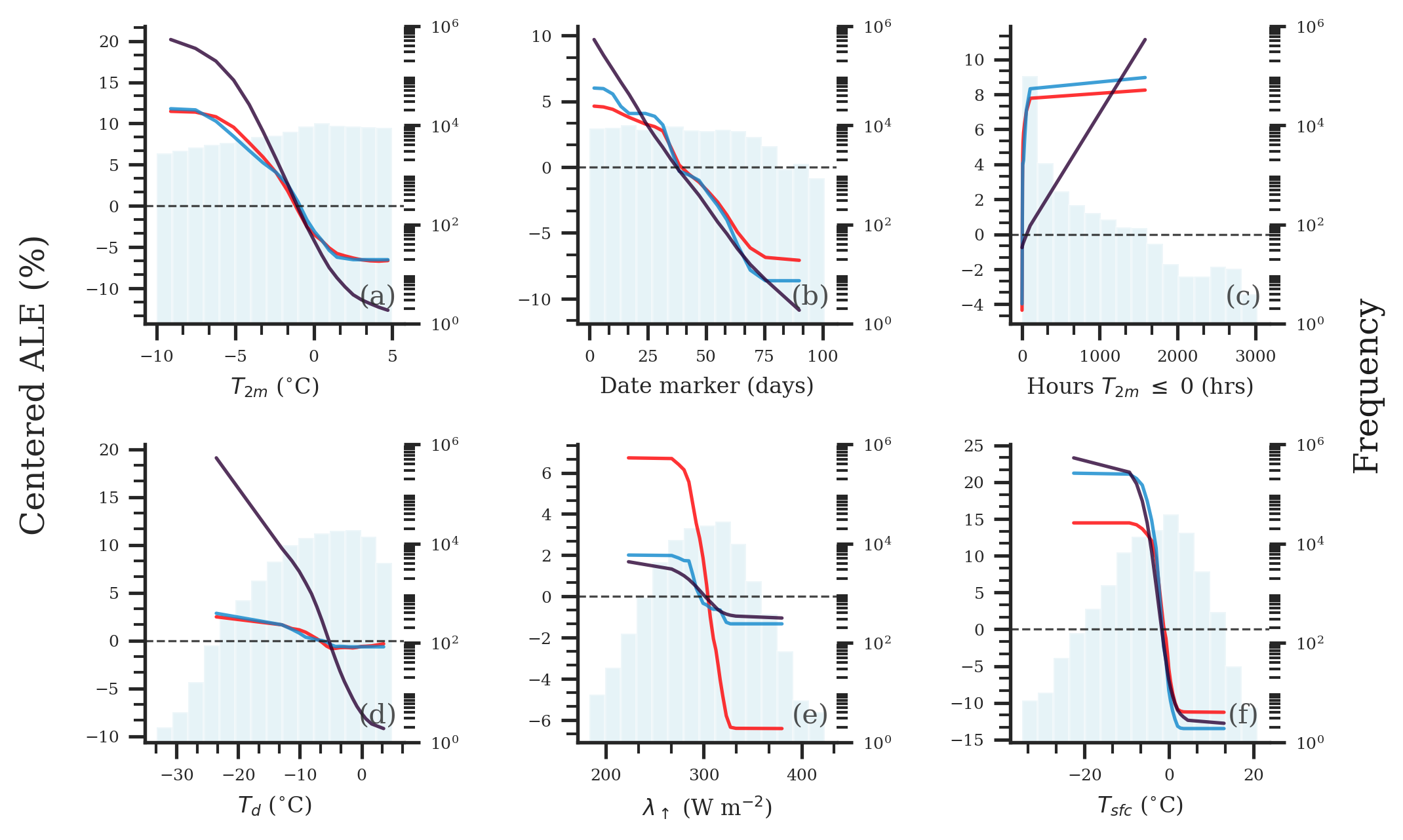
plot_ale(ale=None, features=None, estimator_names=None, add_hist=True, display_feature_names={}, display_units={}, to_probability=None, line_kws={}, cbar_kwargs=None, **kwargs)

Runs the 1D and 2D accumulated local effects plotting.

Parameters

• ale (xarray.Dataset) – Results of ale() for features.

• features (string, list of strings, list of 2-tuple of strings) – Features to plot the PD for. To plot for 2D PD, pass a list of 2-tuples of features.

• estimator_names (string, list of strings (default is None)) – If using multiple estimators, you can pass a single (or subset of) estimator name(s) to plot for.

• add_hist (True/False (default=True)) – If True, adds the histogram of a feature’s values behind the interpret curves.

• display_feature_names (dict) –

  For plotting purposes. Dictionary that maps the feature names in the pandas.DataFrame to display-friendly versions. E.g., display_feature_names = { 'dwpt2m' : '$T_{d}$', }

  The plotting code can handle latex-style formatting.

• display_units (dict) – For plotting purposes. Dictionary that maps the feature names to their units. E.g., display_units = { 'dwpt2m' : '$^\circ$C', }

• line_colors (str or list of strs of len(estimators)) – User-defined colors for curve plotting.

• to_probability (boolean) – If True, the values are multipled by 100.

• matplotlib. (Keyword arguments include arguments typically used for) – E.g., figsize, hist_color,

Returns

fig, axes

Return type

matplotlib figure instance and the corresponding axes

Examples

>>> import skexplain
>>> # pre-fit estimators within skexplain
>>> estimators = skexplain.load_models()
>>> X, y = skexplain.load_data() # training data
>>> explainer = skexplain.ExplainToolkit(estimators=estimators
...                             X=X,
...                             y=y,
...                            )
>>> ale = explainer.ale(features='all')
>>> # Provide a small subset of features to plot
>>> important_vars = ['sfc_temp', 'temp2m', 'sfcT_hrs_bl_frez',
...     'tmp2m_hrs_bl_frez','uplwav_flux']
>>> explainer.plot_ale(ale, features=important_vars)

plot_box_and_whisker(important_vars, example, display_feature_names={}, display_units={}, **kwargs)

Plot the training dataset distribution for a given set of important variables as a box-and-whisker plot. The user provides a single example, which is highlighted over those examples. Useful for real-time explainability.

Parameters

• important_vars (str or list of strings) – List of features to plot

• example (Pandas Series, shape = (important_vars,)) – Single row dataframe to be overlaid, must have columns equal to the given important_vars

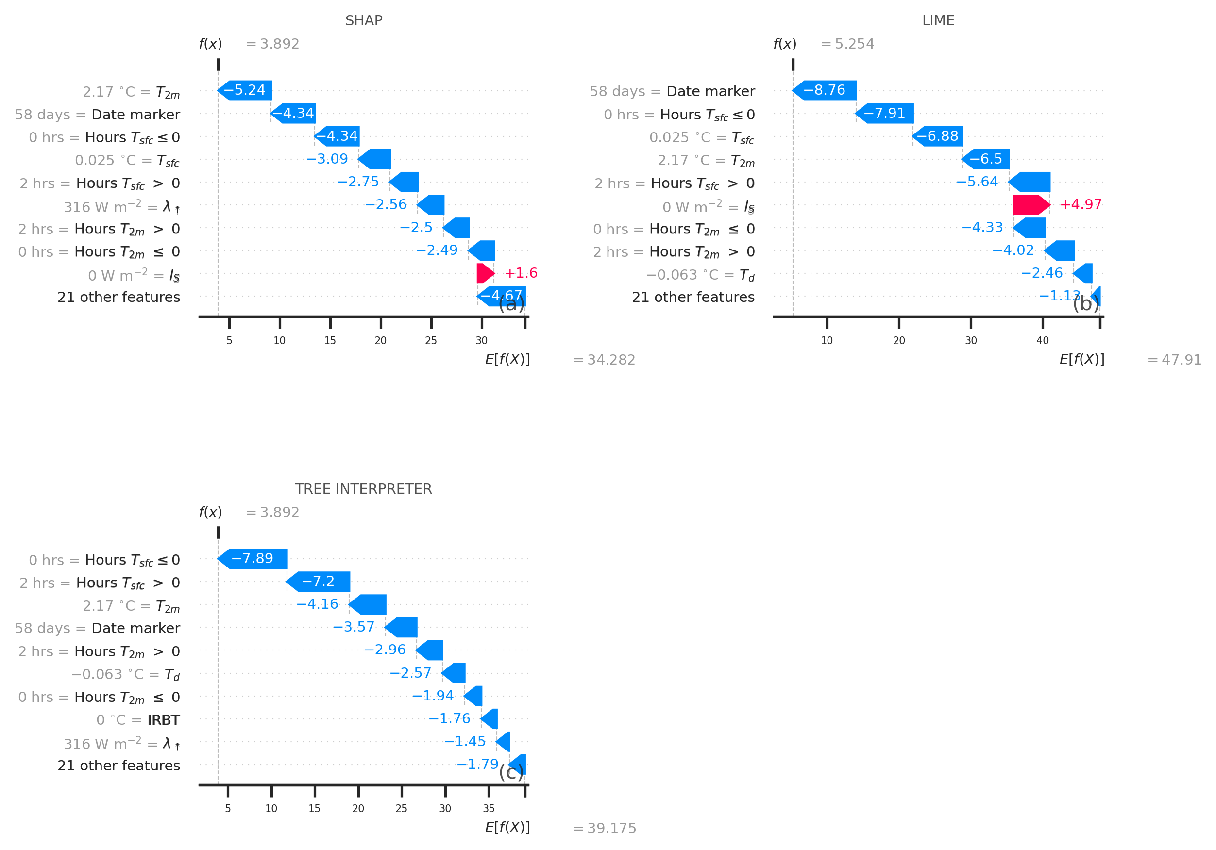
plot_contributions(contrib=None, features=None, estimator_names=None, display_feature_names={}, **kwargs)

Plots the feature contributions.

Parameters

• contrib (Nested pandas.DataFrame or dict of Nested pandas.DataFrame) – Results of local_attributions() or average_attributions() local_attributions() returns an xarray.Dataset which can be valid for multiple examples. For plotting, average_attributions() is used to average attributions and their feature values.

• features (string or list of strings (default=None)) – Features to plot. If None, all features are eligible to be plotted. However, the default number of features to plot is 10. Can be set by n_vars (see keyword arguments).

• estimator_names (string, list of strings (default is None)) – If using multiple estimators, you can pass a single (or subset of) estimator name(s) to compute the IAS for.

• display_feature_names (dict) – For plotting purposes. Dictionary that maps the feature names in the pandas.DataFrame to display-friendly versions. E.g., display_feature_names = { ‘dwpt2m’ : ‘T$_{d}$’, } The plotting code can handle latex-style formatting.

• matplotlib (Keyword arguments include arguments typically used for) –

Returns

fig

Return type

matplotlib figure instance

Examples

>>> import skexplain
>>> import shap
>>> estimators = skexplain.load_models() # pre-fit estimators within skexplain
>>> X, y = skexplain.load_data() # training data
>>> # Only give the X you want contributions for.
>>> # In this case, we are using a single example.
>>> single_example = X.iloc[[0]]
>>> explainer = skexplain.ExplainToolkit(estimators=estimators,
...                             X=single_example,
...                            )
>>> # Create a background dataset; randomly sample 100 X
>>> background_dataset = shap.sample(X, 100)
>>> contrib_ds = explainer.local_contributions(method='shap',
...                   background_dataset=background_dataset)

>>> explainer.plot_contributions(contrib_ds)

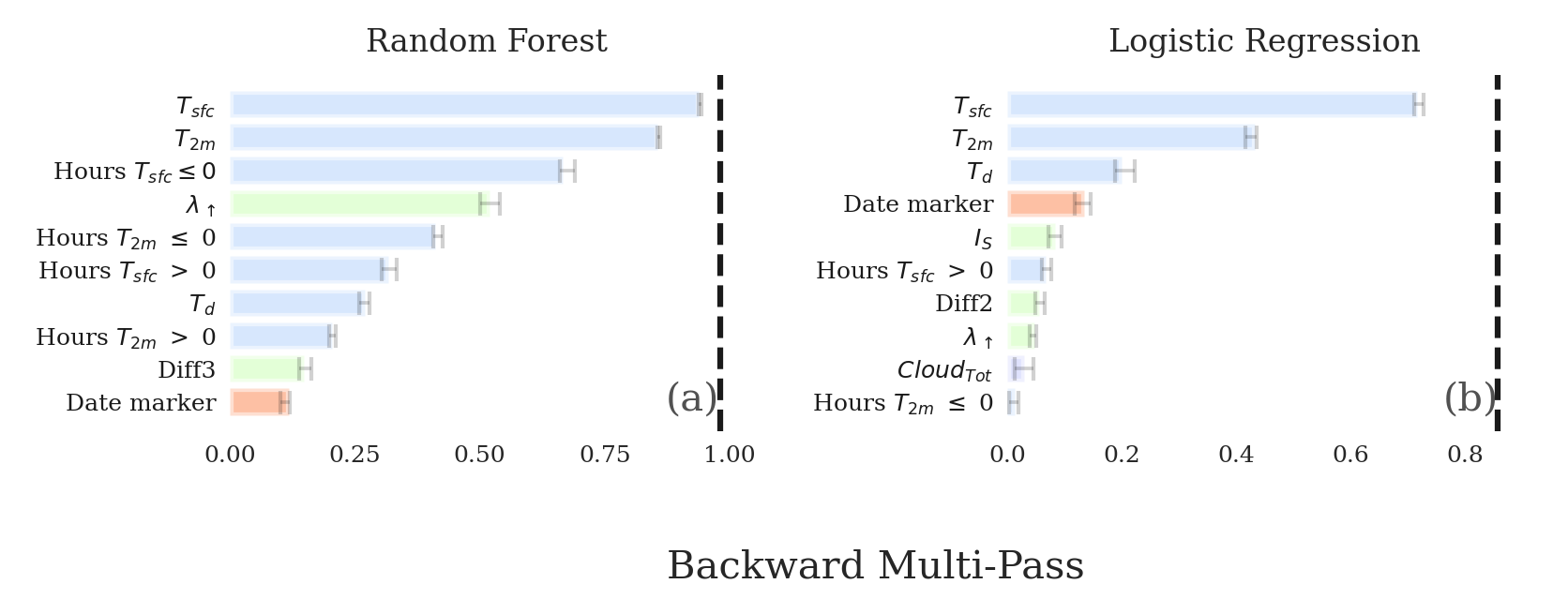
plot_importance(data, panels, plot_correlated_features=False, **kwargs)

Method for plotting the permutation importance and other ranking-based results.

Parameters

• panels (List of 2-tuple of (estimator name, method) to determine the sub-panel) –

  matrixing for the plotting. E.g., If you wanted to compare multi-pass to

  single-pass permutation importance for a random forest:

  panels  = [('Random Forest', 'multipass'), ('Random Forest', 'singlepass')

  The available ranking methods in skexplain include ‘multipass’, ‘singlepass’, ‘perm_based’, ‘ale_variance’, or ‘ale_variance_interactions’.

• data (list of xarray.Datasets) –

  Results from

  • permutation_importance()

  • ale_variance()

  • friedman_h_stat()

  • perm_based_interaction()

  For each element in panels, there needs to be a corresponding element in data.

• columns (list of strings) – What will be the columns of the plot? These can be x-axis label (default is the different estimator names)

• rows (list of strings) – Y-axis label or multiple labels for each row in a multi-panel plot. (default is None).

• plot_correlated_features (boolean) – If True, pairs of features with a linear correlation coefficient > 0.8 are annotate/paired by bars or color-coding. This is useful for identifying spurious rankings due to the correlations.

• kwargs (keyword arguments) –

• num_vars_to_plot (integer) – Number of features to plot from permutation importance calculation.

Returns

fig

Return type

matplotlib figure instance

Examples

>>> import skexplain
>>> # pre-fit estimators within skexplain
>>> estimators = skexplain.load_models()
>>> X, y = skexplain.load_data() # training data
>>> explainer = skexplain.ExplainToolkit(estimators=estimators,
...                             X=X,
...                             y=y,
...                            )
>>> perm_imp_results = explainer.permutation_importance(
...                       n_vars=10,
...                       evaluation_fn = 'norm_aupdc',
...                       direction = 'backward',
...                       subsample=0.5,
...                       n_bootstrap=20,
...                       )
>>> explainer.plot_importance(data=perm_imp_results, method='multipass')

>>> #If we want to annonate pairs of highly correlated feature pairs
>>> explainer.plot_importance(data=perm_imp_results, method='multipass',
...                     plot_correlated_features=True)

plot_pd(pd=None, features=None, estimator_names=None, add_hist=True, display_feature_names={}, display_units={}, to_probability=None, line_kws={}, cbar_kwargs=None, **kwargs)

Runs the 1D and 2D partial dependence plotting.

Parameters

• pd (xarray.Dataset) – Results of pd() for features.

• features (string, list of strings, list of 2-tuple of strings) – Features to plot the PD for. To plot for 2D PD, pass a list of 2-tuples of features.

• estimator_names (string, list of strings (default is None)) – If using multiple estimators, you can pass a single (or subset of) estimator name(s) to plot for.

• add_hist (True/False (default=True)) – If True, adds the histogram of a feature’s values behind the interpret curves.

• display_feature_names (dict) –

  For plotting purposes. Dictionary that maps the feature names in the pandas.DataFrame to display-friendly versions. E.g., display_feature_names = { 'dwpt2m' : '$T_{d}$', }

  The plotting code can handle latex-style formatting.

• display_units (dict) – For plotting purposes. Dictionary that maps the feature names to their units. E.g., display_units = { 'dwpt2m' : '$^\circ$C', }

• line_colors (str or list of strs of len(estimators)) – User-defined colors for curve plotting.

• to_probability (boolean) – If True, the values are multipled by 100.

• matplotlib. (Keyword arguments include arguments typically used for) –

Returns

fig, axes

Return type

matplotlib figure instance and the corresponding axes

Examples

>>> import skexplain
>>> estimators = skexplain.load_models() # pre-fit estimators within skexplain
>>> X, y = skexplain.load_data() # training data
>>> explainer = skexplain.ExplainToolkit(estimators=estimators
...                             X=X,
...                             y=y,
...                            )
>>> pd = explainer.calc_pd(features='all')
>>> # Provide a small subset of features to plot
>>> important_vars = ['sfc_temp', 'temp2m', 'sfcT_hrs_bl_frez',
...     'tmp2m_hrs_bl_frez','uplwav_flux']
>>> explainer.plot_pd(pd, features=important_vars)

plot_scatter(features, kde=True, subsample=1.0, display_feature_names={}, display_units={}, **kwargs)

2-D Scatter plot of ML model predictions. If kde=True, it will plot KDE contours overlays to show highest concentrations. If the model type is classification, then the code will plot KDE contours per class.

save(fname, data, complevel=5, df_save_func='to_json', **kwargs)

Save results of a computation (permutation importance, calc_ale, calc_pd, etc)

Parameters

• fname (string) – filename to store the results in (including path)

• data (ExplainToolkit results) – the results of a ExplainToolkit calculation. Can be a dataframe or dataset.

• complevel (int) – Compression level for the netCDF file (default=5)

• df_save_func ('to_json', 'to_pickle', 'to_csv', 'to_feather', or other str) – The dataframe attribute used to save a pandas dataframe. To use to_feather pyarrow must be installed.

• kwargs (dict) – Args passed to either xarray.Dataset.to_netcdf() (https://docs.xarray.dev/en/stable/generated/xarray.Dataset.to_netcdf.html) or to

Examples

>>> import skexplain
>>> estimators = skexplain.load_models() # pre-fit estimators within skexplain
>>> X, y = skexplain.load_data() # training data
>>> explainer = skexplain.ExplainToolkit(estimators=estimators
...                             X=X,
...                             y=y,
...                            )
>>> perm_imp_results = explainer.calc_permutation_importance(
...                       n_vars=10,
...                       evaluation_fn = 'norm_aupdc',
...                       direction = 'backward',
...                       subsample=0.5,
...                       n_bootstrap=20,
...                       )
>>> fname = 'path/to/save/the/file'
>>> explainer.save(fname, perm_imp_results)

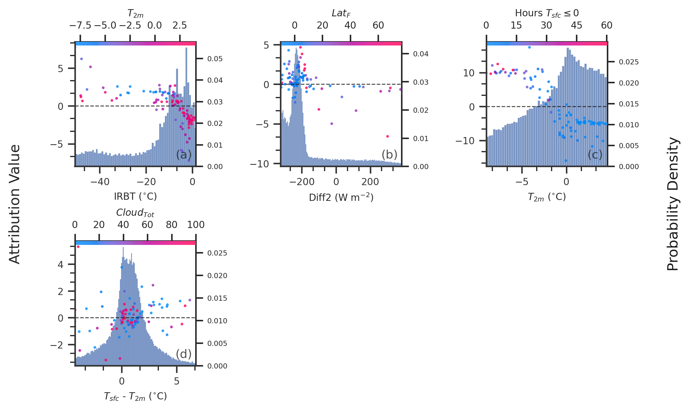
scatter_plot(dataset, estimator_name, method=None, plot_type='summary', features=None, display_feature_names={}, display_units={}, **kwargs)

Plot the SHapley Additive Explanations (SHAP) [13]_ [14]_ [15]_ summary plot or dependence plots for various features.

Parameters

• plot_type ('summary' or 'dependence') – if ‘summary’, plots a feature importance-style plot if ‘dependence’, plots a partial depedence style plot

• dataset (xarray.Dataset) – Results from local_attributions(). Dataset containing feature attribution values, their biases, and the input feature values.

• method ('shap' , 'tree_interpreter', or 'lime' (default is None)) – Can use SHAP, treeinterpreter, or LIME to compute the feature attributions. SHAP and LIME are estimator-agnostic while treeinterpreter can only be used on select decision-tree based estimators in scikit-learn (e.g., random forests). If None, method is determine from the values Dataset. Otherwise, an error is raised.

• features (string or list of strings (default=None)) – features to plots if plot_type is ‘dependence’.

• display_feature_names (dict) – For plotting purposes. Dictionary that maps the feature names in the pandas.DataFrame to display-friendly versions. E.g., display_feature_names = { 'dwpt2m' : '$T_{d}$', } The plotting code can handle latex-style formatting.

• display_units (dict) – For plotting purposes. Dictionary that maps the feature names to their units. E.g., display_units = { 'dwpt2m' : '$^\circ$C', }

• to_probability (boolean) – if True, values are multiplied by 100.

Returns

fig

Return type

matplotlib figure instance

Examples

>>> import skexplain
>>> import shap
>>> # pre-fit estimators within skexplain
>>> estimators = skexplain.load_models()
>>> X, y = skexplain.load_data() # training data
>>> explainer = skexplain.ExplainToolkit(estimators=estimators
...                             X=X,
...                             y=y,
...                            )
>>> # Create a background dataset; randomly sample 100 X
>>> background_dataset = shap.sample(X, 100)
>>> shap_results = explainer.shap(background_dataset)
>>> print(estimator_names)
... ['Random Forest', ]
>>> shap_values, bias = shap_results[estimator_names[0]]
>>> # Plot the SHAP-summary style plot
>>> explainer.plot_shap(plot_type='summary',shap_values=shap_values,)

>>> # Plot the SHAP-dependence style plot
>>> important_vars = ['sfc_temp', 'temp2m', 'sfcT_hrs_bl_frez', 'tmp2m_hrs_bl_frez','uplwav_flux']
>>> explainer.plot_shap(plot_type='dependence',
...            shap_values=shap_values, features=important_vars)

set_X_attribute(X, feature_names=None)

Check the type of the X attribute.

set_estimator_attribute(estimator_objs, estimator_names)

Checks the type of the estimators and estimator_names attributes. If a list or not a dict, then the estimator argument is converted to a dict for processing.

Parameters

• estimators (object, list of objects) – A fitted estimator object or list thereof implementing predict or predict_proba. Multioutput-multiclass classifiers are not supported.

• estimator_names (string, list) – Names of the estimators (for internal and plotting purposes)

set_estimator_output(estimator_output, estimator)

Check the estimator output is given and if not try to assume the correct estimator output.

set_y_attribute(y)

Checks the type of the y attribute.

shap(shap_kws={'algorithm': 'auto', 'masker': None}, shap_kwargs=None)

Compute the SHapley Additive Explanations (SHAP) values [13]_ [14]_ [15]_. By default, we set algorithm = 'auto', so that the best algorithm for a model is determined internally in the SHAP package.

Parameters

shap_kws (dict) –

Arguments passed to the shap.Explainer object. See https://shap.readthedocs.io/en/latest/generated/shap.Explainer.html#shap.Explainer for details. The main two arguments supported in skexplain is the masker and algorithm options. By default, the masker option uses masker = shap.maskers.Partition(X, max_samples=100, clustering=”correlation”) for hierarchical clustering by correlations. You can also provide a background dataset e.g., background_dataset = shap.sample(X, 100).reset_index(drop=True). The algorithm option is set to “auto” by default.

• masker

• algorithm

Returns

results – A dataset containing shap values [(n_samples, n_features)] for each estimator (e.g., ‘shap_values__estimator_name’), the bias (‘bias__estimator_name’) of shape (n_examples, 1), and the X and y values the shap values were determined from.

Return type

xarray.Dataset

References

13

https://christophm.github.io/interpretable-ml-book/shap.html

14

Lundberg, S. M., G. G. Erion, and S.-I. Lee, 2018: Consistent Individualized Feature Attribution for Tree Ensembles. Arxiv,.

15

Lundberg, S. M., and Coauthors, 2020: From local explanations to global understanding with explainable AI for trees. Nat Mach Intell, 2, 56–67, https://doi.org/10.1038/s42256-019-0138-9.

Examples

>>> import skexplain
>>> import shap
>>> # pre-fit estimators within skexplain
>>> estimators = skexplain.load_models()
>>> X, _ = skexplain.load_data() # training data
>>> X_subset = shap.sample(X, 50, random_state=22)
>>> explainer = skexplain.ExplainToolkit(estimators=estimators
...                             X=X_subset,)
>>> results = explainer.shap(shap_kws={'masker' :
...                          shap.maskers.Partition(X, max_samples=100, clustering="correlation"),
...                          'algorithm' : 'auto'})

sobol_indices(n_bootstrap=5000, class_index=1)

Compute the 1st Order and Total order Sobol Indices. Useful for diagnosing feature interactions.

Examples

>>> import skexplain
>>> # pre-fit estimators within skexplain
>>> estimators = skexplain.load_models()
>>> X, y = skexplain.load_data() # training data
>>> explainer = skexplain.ExplainToolkit(estimators=estimators
...                             X=X,
...                             y=y,
...                            )
>>> ale = explainer.ale(features='all')
>>> ias = explainer.interaction_strength(ale)